3 Ways to Freeze Excel Worksheet Rows

Freezing Excel Worksheet Rows: A Step-by-Step Guide
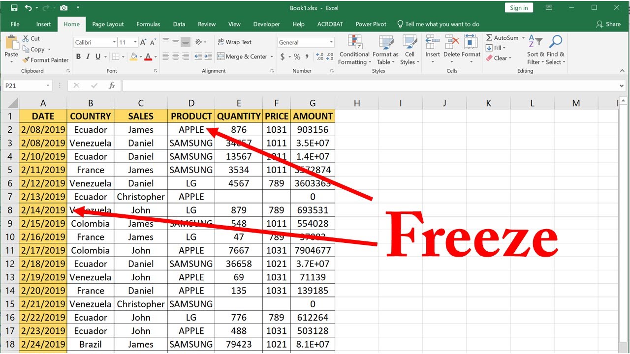
When working with large datasets in Excel, it can be useful to freeze certain rows or columns in place so that they remain visible as you scroll through the worksheet. This can help you keep headers or other important information in view, making it easier to understand and analyze your data. In this article, we’ll explore three ways to freeze Excel worksheet rows.
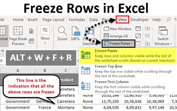
Method 1: Freezing Rows Using the "Freeze Panes" Option
The most straightforward way to freeze rows in Excel is by using the “Freeze Panes” option. Here’s how:
- Select the row below the row(s) you want to freeze.
- Go to the “View” tab in the ribbon.
- Click on “Freeze Panes” in the “Window” group.
- Select “Freeze Panes” again from the dropdown menu.
- Choose “Freeze Top Row” or “Freeze Panes” and select the row(s) you want to freeze.
📝 Note: Make sure to select the row below the row(s) you want to freeze, as this will determine the position of the frozen pane.
Method 2: Freezing Rows Using the "Split" Option
Another way to freeze rows is by using the “Split” option. This method allows you to split the worksheet into separate panes, which can be useful for comparing data or keeping headers in view.
- Select the row below the row(s) you want to freeze.
- Go to the “View” tab in the ribbon.
- Click on “Split” in the “Window” group.
- Adjust the split bar to the desired position.
📝 Note: When using the "Split" option, you can adjust the size of the panes by dragging the split bar.
Method 3: Freezing Rows Using a Macro
If you need to freeze rows frequently, you can create a macro to automate the process. Here’s how:
- Open the Visual Basic Editor by pressing “Alt + F11” or by navigating to “Developer” > “Visual Basic” in the ribbon.
- In the Visual Basic Editor, click “Insert” > “Module” to insert a new module.
- Paste the following code into the module:
Sub Freeze_Top_Row()
    Range("A2").Select
    ActiveWindow.SplitColumn = 0
    ActiveWindow.SplitRow = 1
    ActiveWindow.FreezePanes = True
End Sub
- Save the module by clicking “File” > “Save” (or press “Ctrl + S”).
- To run the macro, go back to the Excel worksheet and press “Alt + F8” to open the Macro dialog box.
- Select the macro and click “Run”.
📝 Note: This macro freezes the top row of the worksheet. You can modify the code to freeze different rows by changing the `Range` and `SplitRow` values.

| Method | Advantages | Disadvantages |
|---|---|---|
| Freeze Panes | Easy to use, flexible | Can be limited in certain situations |
| Split | Allows for multiple panes, adjustable | Can be confusing for beginners |
| Macro | Automates the process, customizable | Requires VBA knowledge, can be complex |
In conclusion, freezing rows in Excel can be a useful feature for keeping important information in view as you work with large datasets. By using one of the three methods outlined in this article, you can easily freeze rows and improve your productivity.
Can I freeze multiple rows in Excel?
+Yes, you can freeze multiple rows in Excel by selecting the row below the rows you want to freeze and using the “Freeze Panes” option.
How do I unfreeze rows in Excel?
+To unfreeze rows in Excel, go to the “View” tab and click on “Freeze Panes” again. Then, select “Unfreeze Panes” from the dropdown menu.
Can I freeze columns in Excel?
+Yes, you can freeze columns in Excel by selecting the column to the right of the column(s) you want to freeze and using the “Freeze Panes” option.


