Match Data in Excel From 2 Worksheets Made Easy
Matching Data in Excel from 2 Worksheets: A Step-by-Step Guide
When working with Excel, there are often instances where you need to match data from two different worksheets. This can be a tedious task, especially if you’re dealing with large datasets. However, with the right techniques and formulas, you can easily match data from two worksheets and streamline your workflow.
In this article, we’ll explore the various methods for matching data in Excel from two worksheets, including using VLOOKUP, INDEX-MATCH, and Power Query.
Method 1: Using VLOOKUP
VLOOKUP is a popular formula in Excel that allows you to search for a value in a table and return a corresponding value from another column. To use VLOOKUP to match data from two worksheets, follow these steps:
- Open your Excel workbook and select the cell where you want to display the matched data.
- Type
=VLOOKUP(and select the value you want to search for. - Select the range of cells that contains the data you want to search, including the column headers.
- Select the column number that contains the data you want to return.
- Type
FALSEto perform an exact match. - Press Enter to execute the formula.
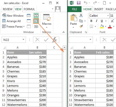
For example, suppose you have two worksheets, “Sheet1” and “Sheet2”, and you want to match the data in column A of Sheet1 with the data in column B of Sheet2. The formula would be:
=VLOOKUP(A2, Sheet2!B:C, 2, FALSE)
This formula searches for the value in cell A2 of Sheet1 in the first column of the range B:C in Sheet2, and returns the corresponding value in the second column.
📝 Note: VLOOKUP can be slow and may not work well with large datasets. It's also sensitive to the order of the columns in the range.
Method 2: Using INDEX-MATCH
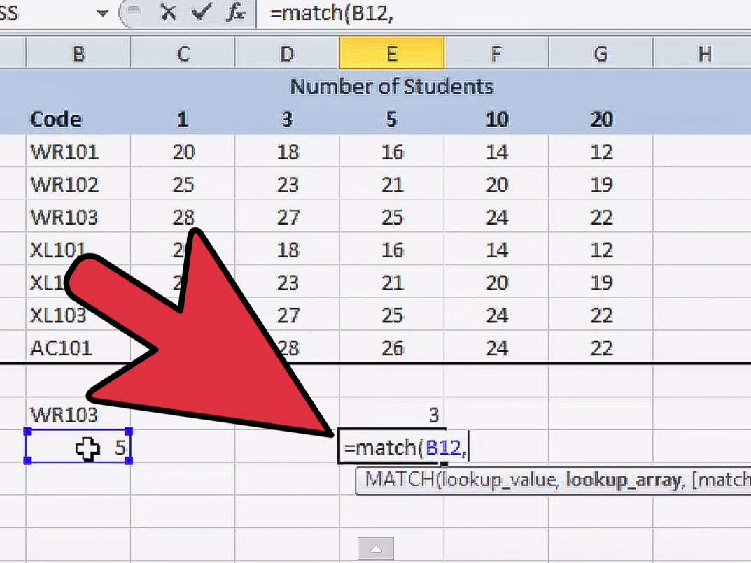
INDEX-MATCH is a more powerful and flexible formula combination that can be used to match data from two worksheets. The INDEX function returns a value at a specified position in a range, while the MATCH function returns the relative position of a value within a range.
To use INDEX-MATCH to match data from two worksheets, follow these steps:
- Open your Excel workbook and select the cell where you want to display the matched data.
- Type
=INDEX(and select the range of cells that contains the data you want to return. - Type
MATCH(and select the value you want to search for. - Select the range of cells that contains the data you want to search.
- Type
, 0)to perform an exact match. - Press Enter to execute the formula.
For example, suppose you have two worksheets, “Sheet1” and “Sheet2”, and you want to match the data in column A of Sheet1 with the data in column B of Sheet2. The formula would be:
=INDEX(Sheet2!C:C, MATCH(A2, Sheet2!B:B, 0))
This formula searches for the value in cell A2 of Sheet1 in the first column of the range B:B in Sheet2, and returns the corresponding value in the second column.
📝 Note: INDEX-MATCH is more flexible and powerful than VLOOKUP, but it can be more complex to use.
Method 3: Using Power Query
Power Query is a powerful data manipulation tool in Excel that allows you to merge and match data from different worksheets. To use Power Query to match data from two worksheets, follow these steps:
- Open your Excel workbook and select the cell where you want to display the matched data.
- Go to the “Data” tab and click on “From Other Sources” > “From Microsoft Query”.
- Select the worksheets you want to merge and match.
- Click on “Merge” and select the common column.
- Click on “OK” to execute the query.
For example, suppose you have two worksheets, “Sheet1” and “Sheet2”, and you want to match the data in column A of Sheet1 with the data in column B of Sheet2. The Power Query formula would be:
=Merge Sheet1!A:B, Sheet2!B:C, "Sheet1!A", "Sheet2!B"
This formula merges the data in column A of Sheet1 with the data in column B of Sheet2, and returns the matched data.
📝 Note: Power Query is a powerful tool that requires some knowledge of data manipulation and query languages.
In conclusion, matching data from two worksheets in Excel can be a challenging task, but with the right techniques and formulas, you can easily achieve it. Whether you use VLOOKUP, INDEX-MATCH, or Power Query, the key is to understand the syntax and limitations of each method.
Here is a summary of the methods:
| Method | Syntax | Limitations |
|---|---|---|
| VLOOKUP | =VLOOKUP(A2, Sheet2!B:C, 2, FALSE) |
Slow, sensitive to column order |
| INDEX-MATCH | =INDEX(Sheet2!C:C, MATCH(A2, Sheet2!B:B, 0)) |
Complex, flexible |
| Power Query | =Merge Sheet1!A:B, Sheet2!B:C, "Sheet1!A", "Sheet2!B" |
Requires knowledge of data manipulation and query languages |
What is the difference between VLOOKUP and INDEX-MATCH?
+VLOOKUP is a formula that searches for a value in a table and returns a corresponding value from another column. INDEX-MATCH is a more powerful and flexible formula combination that can be used to match data from two worksheets. INDEX-MATCH is more flexible and powerful than VLOOKUP, but it can be more complex to use.
What is Power Query?
+Power Query is a powerful data manipulation tool in Excel that allows you to merge and match data from different worksheets. It requires some knowledge of data manipulation and query languages.
Which method is the most efficient?
+The most efficient method depends on the size of the dataset and the complexity of the match. VLOOKUP can be slow and may not work well with large datasets. INDEX-MATCH is more flexible and powerful, but it can be more complex to use. Power Query is a powerful tool that can handle large datasets, but it requires some knowledge of data manipulation and query languages.
